Seismic Facies classification
With several attributes generated for a seismic project, it becomes desirable to integrate the information provided by these attributes, so that they can be interpreted in a convenient and meaningful way. For doing this, some kind of decision making will first need to be done to separate the wheat from the chaff, i.e. the useful features in the seismic attributes are picked up from the background information, for display or further computation. Such decision making could be done either by a human interpreter in an interactive fashion or could be automated with the use of computing machines. Fortunately, a broad range of tools exist that can be used for integrating the information provided by the seismic attributes.
Synonymous with the explosion in the data volumes and compute power that is available these days, the term machine learning has become a buzz word in geoscience, along with deep learning, and others.
Machine learning refers to teaching computers via mathematical operations how to learn from the provided data and make decisions or predictions. As the type of learning style adopted for a given problem to be solved with computers could be specific, it is important to mention it.
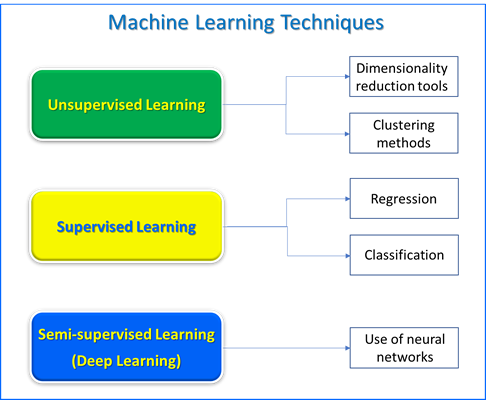
Learning by machines is done in different styles, namely the unsupervised, supervised and the semi-supervised.
Unsupervised learning endeavors to bring out hidden patterns or structure in the volume of input data through pattern recognition algorithms, without any prior knowledge about the desired output.
Supervised learning refers to prior knowledge of the desired output from a subset of the available data input, which is determined through a process called training. Algorithms such as regression, classification, etc. then adopt a pattern identification workflow to predict desired output from the data not used in the training.
Semi-supervised learning adopts the simultaneous use of the prior knowledge on ma small subset of the data, along with a large volume of the data, where no prior information is available. The branch of machine learning that handles such churning of data is referred to as deep learning and makes use of neural networks. Such networks support hidden layers to identify features in the input data to predict the desired outputs.
Under the unsupervised machine learning techniques, clustering methods or dimensionality reduction techniques are commonly used, where the adopted method churns through the seismic data to find patterns and relationships therein. We recommend the application of techniques such as principal component analysis, K-means clustering, self-organized mapping (SOM) and generative topographic mapping (GTM), which help with the study of facies variation with the shale.
We illustrate their application with an example below:
A segment of a section from a seismic volume from the Barents Sea. Time slices at 1280 ms indicated to the left have been extracted from the different attributes and are shown in the figures below. Some of the high-amplitude anomalies seen on the section are associated with channel sands, which we attempt to characterize using some unsupervised machine learning techniques. (Adapted from Chopra and Marfurt (2018); Data courtesy: TGS, Asker)
Time slices generated at 1280 ms from (a) energy-ratio coherence, (b) P-impedance, (c) porosity, and (d) Vclay volumes. The P-impedance volume was generated using prestack simultaneous impedance inversion, and the porosity and Vclay volumes generated using extended elastic impedance. The channels are defined well with the coherence attribute overlaid on the displays (b) to (d) using transparency. Some of the channels exhibiting low impedance, high porosity and low Vclay are indicated with pink arrows. Adapted from Chopra and Marfurt (2018); (Data courtesy: TGS, Asker)
(a) Time slice generated at 1280 ms from (a) K-means clustering co-rendered with coherence using transparency. Equivalent time slice from the first two principal components plotted against a 2D color bar is shown in (b). The 2D color bar as well as the 1D multiplexed 2D color bars are shown in the middle. Similarly, the time slices at 1280 ms from SOM-1 and SOM-2 volume pair, and GTM-1 and GTM-2 volume pair, plotted against a 2D color bar are shown in (c) and (d) respectively. Notice, that while the K-means and principal component displays show the facies distribution within the channels, there is better distribution of the channel facies on the SOM display (channel to the left indicated with cyan arrow). The most detailed distribution of channel facies and their distinct definition is seen on the GTM display. (Adapted from Chopra and Marfurt (2018); ta courtesy: TGS, Asker)
References
Chopra, S., and K. J. Marfurt, 2018, Seismic facies classification using some unsupervised machine learning methods, 88th Annual International Meeting, SEG, Expanded Abstracts, 2056-2060.


